Machine Learning Turns AUV Acoustics Into 2 m Nodule Maps

Title: An Interpretable Multi-Model Machine Learning Approach for Spatial Mapping of Deep-Sea Polymetallic Nodule Occurrences
Authors: Iason-Zois Gazis, Francois Charlet, and Jens Greinert
Journal & Year: Natural Resources Research, 2024
BLUF: High-resolution autonomous underwater vehicle mapping in the eastern Clarion Clipperton Zone shows that multibeam backscatter, especially the 25 to 55 degree mean-far angular band, together with simple terrain metrics, predicts percent nodule coverage at 2 m resolution. A random forest explained 84 percent of the variance on an independent 20 percent image test set, and variable-importance analyses across five algorithms consistently ranked multibeam backscatter as the top predictor. Over 37.34 km² at 2 m pixels, the team delivers a transferable and interpretable workflow that can tighten resource estimates, guide collector path planning, and help position ecological baselines with clearer model auditability.
Patchy nodule distribution complicates both economic tonnage estimation and habitat assessment. Gazis et al. combined more than 31,000 annotated AUV photographs with 400 kHz multibeam echosounder data, 230 kHz side scan sonar mosaics, and a suite of geomorphological derivatives to learn continuous nodule coverage surfaces. They trained and compared five supervised algorithms (generalized linear and additive models, support vector machines, random forests, and neural networks), emphasizing interpretability through variable importance, partial dependence plots, and area of applicability maps.
Data and methods at a glance:
- Survey footprint: 37.34 km² were mapped. Multibeam echosounder (MBES, a sonar that measures seafloor depth and acoustic hardness) and side scan sonar (SSS, a sonar that pictures seafloor texture) products are at 2 m resolution. Orthophoto mosaics (stitched, geometrically corrected color photos) are at 2 mm, and digital elevation models (DEMs, 3D seafloor height grids) are at 5 mm.
- Ground truth: 31,409 AUV stills, auto-segmented for percent cover.
- Predictors: MBES bathymetry and derivatives (slope, BPI, eastness), MBES backscatter mosaic, angle-resolved backscatter statistics and inversions (impedance, volume), SSS backscatter and Local Moran texture metrics.
- Modeling strategy: Stratified 80-20 train-test split, then spatial cross validation with 3 by 3 km blocks chosen from a formal autocorrelation and feature-space representativeness analysis, hyperparameter tuning inside the spatial folds, and area of applicability mapping to flag extrapolation.
Predicted coverage patterns closely matched the test images and box corer data; the random forest generalized best overall (test R2 = 0.84). However, it compressed the value range, underestimating highs and overestimating lows, while SVM produced isolated unrealistic 100 percent pixels.
Figure 9(b) is the clearest single visual: it ranks the mean far 25 to 55 degree angular backscatter band as the most important predictor and shows, via partial dependence, the strongest monotonic rise in predicted nodule cover with increasing backscatter, which is why MBES backscatter is highlighted as the primary driver.
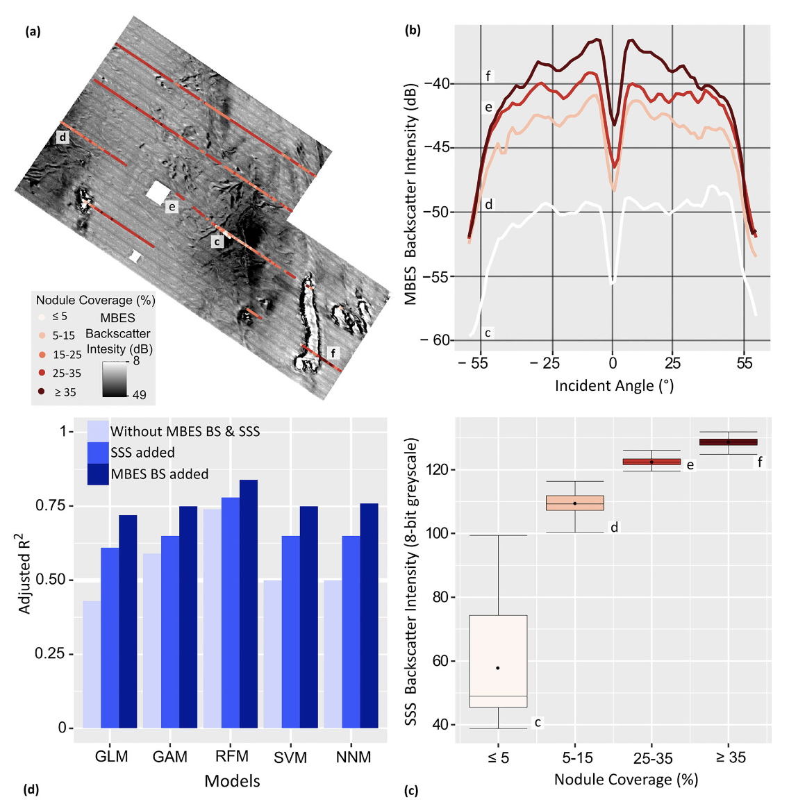
Angle-resolved backscatter was decisive. Differences in MBES backscatter exceeded 5 dB between nodule-poor and nodule-rich patches, with the mean-far 25 to 55 degree band carrying the strongest signal. The paper does not report a specific dB threshold at which coverage rises sharply.
Terrain mattered, especially when hydroacoustic predictors were withheld. Coverage peaked on relatively flat seabed with slopes under about 3 degrees and on east-facing slopes. The authors attribute these spatial relations to the prevailing northwestward bottom currents in the area, rather than a westward flow. Local depressions and steep gullies showed low coverage.
Across models, removing the hydroacoustic predictors markedly reduced skill, but the paper does not quantify the loss as one third. Adding SSS backscatter improved performance, particularly for simpler models.
Near-bottom AUV acoustics can pre-screen high grade nodule tracts before dense coring, and partial dependence plus area of applicability diagnostics let engineers and regulators see where and why the model is confident or extrapolating. Planning can prioritize flat, east-facing slopes that the models consistently rank higher, while routing cautiously around cliffs, troughs, and sediment sinks that forced all models to extrapolate.


